5. Calibration
This chapter describes how gas measurements in kOhm and ppb are translated to the standardized and ‘better interpretable’ units of ug/m3 (microgram per cubic meter).
The challenge is that Jose sensors produce noisy and biased measurements of gas components on a wrong scale. The data is noisy because two consecutive measurements of the same gas component can vary a lot. The measurements are biased because the gas sensors are cross sensitive for (at least) temperature and other gas components. The measurements are on the wrong scale because the results in kOhm instead of the more interpretable ug/m3 or ppm. These issues are fixed by calibrating the Jose sensors to reliable RIVM measurements.
Data from Jose and RIVM is pre-processed before using it to train an Artificial Neural Network (ANN). The performance is optimized and the best model is chosen for online predictions.
These processes were initially executed manually. At a later stage, and thus currently, the entire ANN Calibration process is automated.
The idea to use ANN emerged when initial calibration using Linear Regresssion-based methods did not render satisfactory results. From studying existing research like
- “Field calibration of a cluster of low-cost available sensors for air quality monitoring” by Spinelle, Gerboles et al
- “Air Temperature Estimation by Using Artificial Neural Network Models in the Greater Athens Area, Greece” by A. P. Kamoutsis et al.
ANN appeared a good candidate. Though complex when manually performed, we also aimed to overcome this by automating both the learning and calibration process within the already existing SE ETL process pipelines.
5.1. Data
Data used for calibration (training the ANN) originates from Jose (raw data) and RIVM (reference data) stations that are located pairwise in close proximity. They are located at the Graafseweg and Ruyterstraat in Nijmegen.
Data was gathered for a period of february 2016 to now.
Data was initially manually delivered:
- RIVM reference data by Jan Vonk (RIVM).
- Raw data from the Jose sensors by Robert Kieboom (CityGIS).
At a later stage, and thus currently, this data delivery is automated and continuous:
- RIVM data is harvested from the public RIVM LML SOS via the ETL Harvester_rivm
- Jose data is harvested from the Whale Server(s) via the ETL Harvester and then further extracted via the ETL Extractor
The overal datastream is depicted in Figure 1 below.
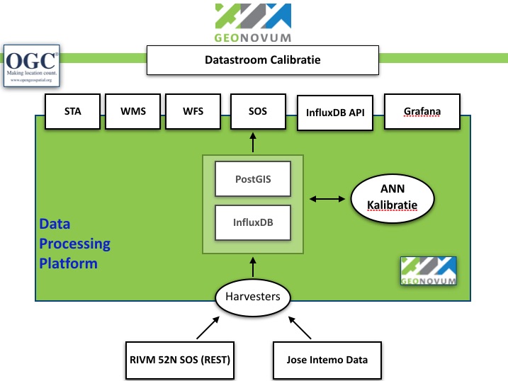
Figure 1 - Overall setup ANN calibration
The harvested RIVM SOS data provides aggregated hour-records. Data from the Jose sensors have irregularities due to lost wifi connection or power issues. Figure 2 below shows the periods of valid gas measurements taken by Jose sensors.
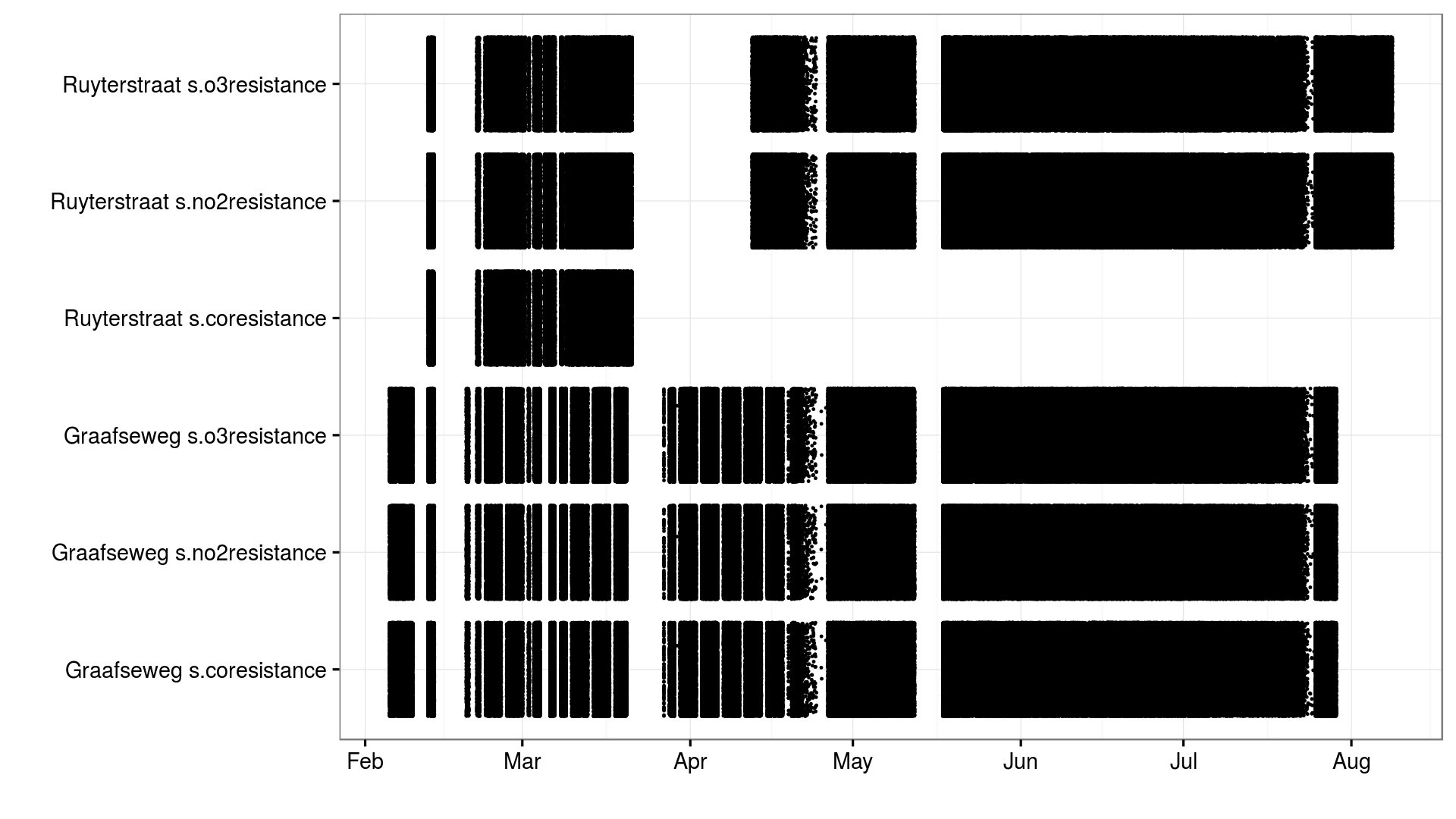
Figure 2 - Valid gas measurements taken by Jose sensors
5.2. Pre-processing
Before using the data form Jose and RIVM it needs to be pre-processed:
- Erroneous measurements are removed based on the error logs from RIVM and Jose.
- Extremely unlikely measurements are removed (e.g. gas concentrations below 0)
- The RIVM data is interpolated to each time a Jose measurement was taken.
- The RIVM data is merged with the Jose data. For each Jose measurement the corresponding RIVM measurements are now known.
- A rolling mean is applied to the gas components of the Jose data. Actually this step is done during the parameter optimization to find out which length of rolling mean should be used.
- A random subset of 10% of the data is chosen to prevent redundant measurements. Actually this step is done during the parameter optimization.
The pre-processing was initially done in R, later in Python (see below).
5.3. Neural Networks
There are several options to model the relationship between the Jose measurements and RIVM measurements. In this project a Feed-forward Neural Network is used. Its advantage is that it can model complex non-linear relations. The disadvantage is that understanding the model is hard.
A neural network in general can be thought of as a graph (see Figure 2). A graph contains nodes and edges. The neural network specifies the relation between the input nodes and output nodes by several edges and hidden layers. The values for the input nodes are clamped to the independent variables in the data set, i.e. the Jose measurements. The neural network should adapt the weights of each of the edges such that the value of the output node is as close as possible to the dependent variable, i.e. the RIVM measurement.
The hidden nodes take a weighted average (resembled by de edges to each of the inputs) and then apply an activation function. The activation function squashes the weighted average to a finite range (e.g. [-1, 1]). This allows the neural network to transform the inputs in a non-linear way to the output variable.
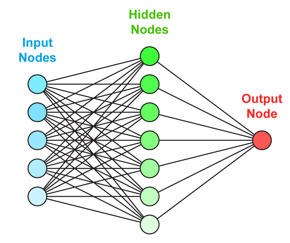
Figure 3 - The structure of a Feed-forward Neural Network can be visualized as a graph
5.4. Training a Neural Network
A neural network is completely specified by the the weights between the nodes and the activation function of the nodes. The latter is specified on beforehand and thus only the weights should be learned during the training phase.
There is no way to find the optimal weights in an efficient way for an arbitrary neural network. Therefore, a lot of methods are proposed to iteratively approach the global optimum.
Most of them are based on the idea of back-propagation. With back-propagation the error for each of the records in the data is used to change the weights slightly. The change in weights makes the error for that specific record lower. However, it might increase the error on other records. Therefore, only a tiny alteration is made for each error in each record.
As an addition the used L-BFGS method also uses the first and second derivatives of the error function to converge faster to a solution.
5.5. Performance evaluation
To evaluate the performance of the model the Root Mean Squared Error (RMSE) is used. The RMSE is the average error (prediction - actual value) of the model. Lower RMSE values are better.
Testing the model on the same data as it is trained on could lead to over-fitting. This means that the model learn relations that are not there in practice. For this reason the performance evaluation needs to be done on different data then the learning of the model. For example, 90% of the data is used to train the model and 10% is used to test the model. This process can be repeated when using a different 10% to test the data. With the 90%-10% ratio this process can be repeated 10 times. This is called cross validation. In practice, cross validation with 5 different splits of the data is used.
5.6. Parameter optimization
Training a neural network optimizes the weights between the nodes. However, the training process is also susceptible to parameters. For example, the number of hidden nodes, the activation function of the hidden nodes, the learning rate, etc. can be set. For a complete list of all the parameters see the documentation of MLPRegressor.
Choosing different parameters for the neural network learning influences the performance and complexity of the model. For example, using to few hidden nodes results in a model that cannot fit the pattern in the data. On the other hand, using to many hidden nodes may model relationships that are to complex and do not generalize to unseen data.
Parameter optimization is the process of evaluating different parameters. RandomizedSearchCV from sklearn is used to try different parameters and evaluate them using cross-validation. This method trains and evaluates a neural network n_iter times. The actual code looks like this:
gs = RandomizedSearchCV(gs_pipe, grid, n_iter, measure_rmse, n_jobs=n_jobs,
                        cv=cv_k, verbose=verbose, error_score=np.NaN)
gs.fit(x, y)
The first argument gs_pipe is the pipeline that filters the data and applies a neural network, grid is a collection with distributions of possible parameters, n_iter is the number of parameters to try, measure_rmse is a function that computes the RMSE performance and cv_k specifies the number of cross-validations to run for each parameter setting. The other parameters control the process.
5.7. Choosing the best model
A good model has a good performance but is also as simple as possible. Simpler models are less likely to over-fit, i.e simple models are less likely to fit relations that do not generalize to new data. For this reason, the simplest model that performs about as well (e.g. 1 standard deviation) as the best model is selected.
For each gas component this results in models with different learning parameters. Differences are in the size of the hidden layers, the learning rate, the regularization parameter, the momentum and the activation function . For more information about these parameters check the documentation of MLPRegressor. The parameters for each gas component are listed below:
CO_final = {'mlp__hidden_layer_sizes': [56],
            'mlp__learning_rate_init': [0.000052997],
            'mlp__alpha': [0.0132466772],
            'mlp__momentum': [0.3377605568],
            'mlp__activation': ['relu'],
            'mlp__algorithm': ['l-bfgs'],
            'filter__alpha': [0.005]}

O3_final = {'mlp__hidden_layer_sizes': [42],
            'mlp__learning_rate_init': [0.220055322],
            'mlp__alpha': [0.2645091504],
            'mlp__momentum': [0.7904790613],
            'mlp__activation': ['logistic'],
            'mlp__algorithm': ['l-bfgs'],
            'filter__alpha': [0.005]}

NO2_final = {'mlp__hidden_layer_sizes': [79],
             'mlp__learning_rate_init': [0.0045013008],
             'mlp__alpha': [0.1382210543],
             'mlp__momentum': [0.473310471],
             'mlp__activation': ['tanh'],
             'mlp__algorithm': ['l-bfgs'],
             'filter__alpha': [0.005]}
5.8. Online predictions
The sensorconverters.py converter has routines to refine the Jose data. Here the raw Jose measurements for meteo and gas components are used to predict the hypothetical RIVM measurements of the gas components.
Three steps are taken to convert the raw Jose measurement to hypothetical RIVM measurements.
The measurements are converted to the units with which the model is learned. For gas components this is kOhm, for temperature this is Celsius, humidity is in percent and pressure in hPa.
A rolling mean removes extreme measurements. Currently the previous rolling mean has a weight of 0.995 and the new value a weight of 0.005. Thus alpha is 0.005 in the following code:
def running_mean(previous_val, new_val, alpha):
    if new_val is None:
        return previous_val

    if previous_val is None:
        previous_val = new_val
    val = new_val * alpha + previous_val * (1.0 - alpha)
    return val
For each gas component a neural network model is used to predict the hypothetical RIVM measurements. Prediction are only made when all gas components are available. The actual prediction is made with this code:
# Predict RIVM value if all values are available
if None not in [o3, no2, co2, temp_amb, temp_unit, humidity, baro]:
    value_array = np.array([baro, humidity, temp_amb, temp_unit, gasses['co2'], gasses['no2'], gasses['o3']])
    val = pipeline_objects[gas].predict(value_array.reshape(1, -1))[0]

return val
5.9. Results
Calibrated values are also stored in InfluxDB and can be viewed using Grafana. Login with name user and password user.
See an example in Figure 5 and 6 below. Especially in Figure 5, one can see that calibrated values follow the RIVM reference values quite nicely. More research is needed to see how the ANN is statistically behaves.
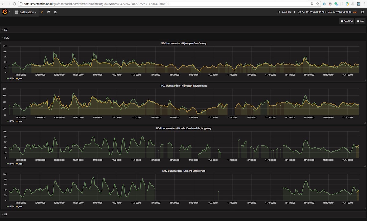
Figure 5 - Calibrated and Reference values in Grafana
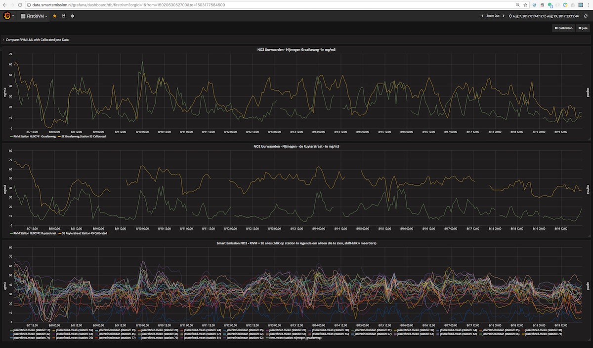
Figure 6 - Calibrated and Reference values in Grafana
5.10. Implementation
The implementation of the above processes is realized in Python. Like other ETL within the Smart Emission Platform, the implementation is completely done using the Stetl ETL Framework. The complete implementation can be found in GitHub.
Four Stetl ETL processes realize the three phases of ANN Calibration:
- Data Harvesting - obtaining raw (Jose) and reference (RIVM) data (2 processes)
- Calibrator - the ANN learning process, providing/storing the ANN Model (in PostGIS)
- Refiner - actual calibration using the ANN Model (from PostGIS)
Data Harvesting and Refiner are scheduled (via cron) continously. The Calibrator runs “once in a while”.
5.10.1. Data Harvesting
The Harvester_rivm ETL process obtains LML measurements records from the RIVM SOS. Data is stored in InfluxDB.
The standard SE Harvester already obtains raw data from the Whale servers and stores this data in the PostGIS DB. To make this data better accessible the Extractor selects (not all data goes through ANN) and obtains raw measurements (gases and others like meteo) records from the PostGIS DB and puts this data in InfluxDB.
The result of Data Harvesting are two InfluxDB Measurements collections (tables) with timeseries representing the raw (Jose) and reference (RIVM) data.
5.10.2. Calibrator
The Calibrator takes as input the two InfluxDB Measurements (tables): rivm (reference data) joseraw (Raw Jose data). Here “the magic” is performed in the following steps:
- merging the two datastreams in time
- performing the learning process
- storing the result ANN model in PostGIS
5.10.3. Refiner
This process takes raw data from the harvested timeseries data. By updating the sensordefs object with references to the ANN model the raw data is calibrated via the sensorconverters and stored in PostGIS.